
Beyond Poisson: Modeling Bursty and Correlated Arrivals in Google Cloud Workloads
目次

 Background and Motivation
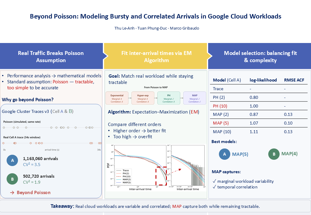
Modern data centers, running millions of cloud computing and AI/ML jobs every day, need accurate performance analysis to optimize resource allocation. The standard mathematical tool for this is queueing theory, which requires input distributions that are mathematically tractable.
The most common assumption is a Poisson process for job inter-arrival times. The problem: this assumption does not reflect reality. Analyzing real data from Google Cluster Traces, we found that job inter-arrival times are:
- Highly variable
- Heavy-tailed — occasionally producing very long gaps between jobs
- Temporally correlated — arrivals are not independent of one another
These three properties mean that Poisson, and even more flexible models like the hyper-exponential distribution, cannot adequately capture real workload behavior.
Related Work
- Leland et al. (1993) made a landmark discovery: Ethernet traffic exhibits self-similarity — burstiness persists across every time scale, rather than smoothing out as Poisson models predict.
- Feldmann & Whitt (1998) proposed fitting heavy-tailed distributions (Pareto, Weibull) and converting them into a hyper-exponential form for tractable analysis.
- Khayari et al. (2003) improved this by fitting hyper-exponential distributions directly via the EM (Expectation-Maximization) algorithm, removing the intermediate conversion step.
- Yildiz & Baiocchi (2024) fitted two-phase hyper-exponential distributions to Google trace data, but found something important: the fitted model matched shuffled traces better than the original sequence — revealing that matching the marginal distribution alone misses the temporal correlation structure.
- Other approaches use machine learning (K-Means clustering, GANs) to generate synthetic workloads. While realistic, these are computationally expensive black-box models that don’t provide explicit distributional forms — which analytical queueing models need.
The gap: we need a model that is flexible enough to fit real data, stays mathematically tractable, and captures temporal correlation — something hyper-exponential cannot do.
We therefore fit two model classes:
- Phase-type (PH) distributions — a generalization of hyper-exponential, far more flexible.
- Markovian Arrival Process (MAP) — an extension of PH that retains “memory” between consecutive arrivals, enabling it to capture correlation.
Data Used
Source: Google Cluster Traces v3 — 8 clusters (“cells”) across North America, Europe, and Asia, recorded in May 2019. Each cell contains roughly 12,000 machines.
Inter-arrival time (IAT) = elapsed time between consecutive job submissions within a cell.
Data preprocessing (based on a cleaned version released by Yildiz et al.):
-
- Removed tasks starting/ending outside the observation window (avoiding boundary effects).
- Removed tasks with zero CPU/memory usage (no documented explanation for such anomalies).
- Kept only tasks with “FINISH” status — excluding “KILL,” “LOST,” and “FAIL” tasks, since their recorded duration/resource usage may not reflect actual job requirements.
- Filtered-out tasks accounted for less than 1% of the dataset.
We focused on Cell A and Cell B, chosen for their contrasting characteristics:
-
- Cell A: higher variability (CV² = 3.52)
- Cell B: longer inter-arrival times with a heavier tail (CV² = 1.92, larger absolute mean/median)
Table 1: Statistics of inter-arrival times (seconds)
| Trace | Mean | Median | CV² | 99th percentile | Max |
| Cell A | 2.30 | 0.47 | 3.52 | 20.57 | 164.00 |
| Cell B | 5.33 | 2.54 | 1.92 | 34.18 | 125.21 |
Both traces show mean ≫ median (right-skewed) and CV² > 1 — variability far beyond what an exponential distribution (CV² = 1) could represent.
Modeling Approach
Step 1 — Baseline: Exponential & Hyper-exponential (Method of Moments)
- Exponential: a single parameter fully determined by the sample mean — too simple, decays too fast, misses the heavy tail entirely.
- Hyper-exponential: more flexible, substantially improves the tail fit — but discrepancies remain at extreme values (near-zero and very large inter-arrival times), showing that low-order hyper-exponential models still lack flexibility.
- Technical note: hyper-exponential parameters were estimated via Method of Moments (MoM) rather than EM, since EM tends to produce degenerate solutions with extreme rate parameters for this model.
Step 2 — Advanced models: Phase-type (PH) & MAP via the EM algorithm
We used the Expectation-Maximization (EM) algorithm — a maximum-likelihood method for models with latent (unobserved) structure, iterating between:
- E-step: compute the conditional expectation of the complete-data log-likelihood, given the observed data and current parameters.
- M-step: update parameters to maximize this expected log-likelihood.
For PH and MAP, the latent variable is the hidden phase evolution of the underlying continuous-time Markov chain (i.e., the transition counts and time spent in each phase). Implemented via BuTools 2.
Results and Proposal
Cell A results
| Model | Log-likelihood | Moment 2 | Moment 3 | RMSE ACF |
| PH(2) | 0.80 | 15.01 | 146.69 | – |
| PH(10) | 1.00 | 21.35 | 302.50 | – |
| MAP(2) | 0.87 | 15.01 | 146.65 | 0.13 |
| MAP(5) | 1.07 | 22.41 | 373.50 | 0.10 |
| MAP(10) | 1.11 | 21.95 | 333.68 | 0.13 |
- PH(10) matches the marginal distribution almost perfectly.
- Increasing MAP order only marginally improves the tail fit — but MAP’s real advantage is capturing temporal correlation, which PH cannot.
- MAP(10) has the highest log-likelihood but is NOT the best model overall — it fits moments worse than MAP(5) and has a worse (higher) ACF RMSE, signaling overfitting.
- MAP(5) offers the best balance for Cell A: lowest ACF RMSE (0.10) while keeping high log-likelihood and good moment matching.
Cell B results
| Model | Log-likelihood | Moment 2 | Moment 3 | RMSE ACF |
| PH(2) | −2.43 | 60.42 | 1027.72 | – |
| PH(4) | −2.06 | 82.96 | 2079.82 | – |
| MAP(2) | −2.36 | 71.51 | 1449.19 | 0.06 |
| MAP(3) | −1.94 | 74.48 | 1603.78 | 0.05 |
| MAP(4) | −1.92 | 80.18 | 1950.44 | 0.05 |
- Both PH and MAP achieve good fits at lower orders for Cell B.
- PH(4) closely matches the empirical marginal distribution.
- MAP(4) is the optimal choice: highest log-likelihood, good moment matching, lowest ACF RMSE — while further increasing the order beyond MAP(3) brings only marginal gains, not worth the added complexity.
Conclusions
- Real Google data center workloads go far beyond the Poisson assumption — they are highly variable, heavy-tailed, and temporally correlated.
- PH distributions fit the marginal distribution very well but cannot capture correlation (being a renewal process).
- MAP offers the best balance: nearly matches PH’s marginal fit while also capturing temporal correlation — critical for real-world performance analysis and capacity planning.
Moderate-order models give the best results, avoiding both underfitting and overfitting.
Afterword
One of the biggest challenges in this project was that real world data does not behave like the parametric distributions typically assumed in queueing models. Google’s job arrivals are bursty and irregular, not smooth and memoryless like an idealized Poisson process, so before any fitting could begin, we had to test and compare many candidate models rather than assume one would simply work.
No single distribution fit the data perfectly. Across repeated tests, however, MAP consistently outperformed the alternatives, particularly in capturing the temporal correlation that simpler models missed entirely. Finding the right model order was equally important: increasing the order too far did not translate into a better model. It mainly added complexity and led to overfitting, without meaningfully improving the fit to real system behavior.
I’m grateful to Prof. Tuan Phung Duc, my supervisor at the University of Tsukuba, and Prof. Marco Gribaudo, my advisor at Politecnico di Milano, for their guidance throughout this work. I am currently continuing this collaboration with Prof. Gribaudo and his research group, extending the modeling approach to LLM workload data collected by his team.
References
- Leland, W.E., Taqqu, M.S., Willinger, W., Wilson, D.V.: On the self-similar nature of Ethernet traffic. In: Conference proceedings on Communications architectures, protocols and applications, pp. 183–193 (1993)
- Feldmann, A., Whitt, W.: Fitting mixtures of exponentials to long-tail distributions to analyze network performance models. Performance Evaluation 31(3-4), 245–279 (1998)
- Khayari, R.E.A., Sadre, R., Haverkort, B.R.: Fitting World-Wide Web request traces with the EM-algorithm. Performance Evaluation 52(2-3), 175–191 (2003)
- Horváth, G., Telek, M.: BuTools 2: a rich toolbox for Markovian performance evaluation. In: Valuetools, vol. 16, pp. 137–142 (2016)
- Yildiz, M., Baiocchi, A.: Data-driven workload generation based on Google data center measurements. In: 2024 IEEE 25th International Conference on High Performance Switching and Routing (HPSR), pp. 143–148 (2024)
- Wilkes, J.: Cluster data 2019 (2019), https://github.com/google/cluster-data
Cases in the same field
-

Enhancing System Reliability via Multi-Version Machine Learning and Rejuvenation ― A Case Study on Multi-Version Perception with Time-Triggered Rejuvenation in an AV Simulator
TrafficClassification2026/03/31
-

Can One Deep-Learning Detector Find Trees Across Any LiDAR Platform?
Information-and-communicationEnvironmentNatural-scienceModelingPredictionFeature-extraction2026/03/25
-

Effect of Elimination of Electricity Poles from the Viewpoint of Disaster Mitigation and Off-grid Power Supply – Using Electricity Pole Positional Data for the South of the Prefecture –
PlanEffect-verificationOptimization2021/07/16

